Solutions to problems from IOI 2018

Here I present a detailed description how to solve all six problems from the International Olympiad in Informatics 2018 which was held in Tsukuba, Japan. This work was partially funded by the International Committee of IOI.

The problems are Combo, Werewolf, Seats (from the first day of the competition), and Mechanical Doll, Highway Tolls, Meetings (from the second day). Full problem statements (as well as test data used to judge contestants' solutions) are available at the official webpage of the competition. All programs described in this article are available on my GitHub repository.

Combo

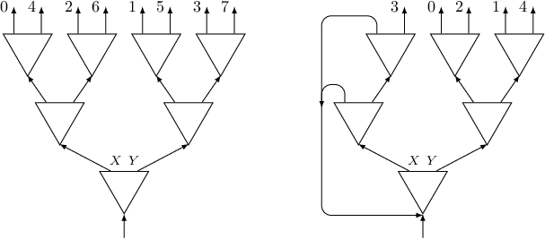
In this problem there is a secret string $S$ of length $N$ which consists of four characters (namely $A$, $B$, $X$ and $Y$). We also know that the first character of the string never reappears in it. Our task is to determine the string by using at most $N+2$ guesses. In each guess we specify a string $G$ of length at most $4N$ consisting of above four characters, and we get the maximum length of a prefix of $S$ which is a substring of $G$.

Let's try some sample. Suppose that $N=3$, and we make our first guess of $G = ABX$. Let's see what answers we could get. If the answer is $3$, then it means we are lucky – there is only one substring in $G$ of length $3$ (the whole string) and it is a prefix of $S$, so $S=ABX$ and we are done. But probably we won't be so lucky in our first guess. If the answer is $2$, then it means that either $AB$ or $BX$ is a prefix of $S$, thus $S = AB?$ or $S = BX?$. If the answer is $1$, then it means that either $A$, $B$ or $X$ is a prefix of $S$, so we know that the first letter of $S$ is either $A$, $B$ or $X$. Finally, if the answer is $0$, that means that the first letter of $S$ must be $Y$.

First attempt – guessing exactly one prefix

It's hard to guess the whole string, but we can start small, and try to guess some shorter prefix of $S$ – maybe just one letter? In order to do that, we can ask $4$ guesses: $G=A$, $G=B$, $G=X$ and $G=Y$. Exactly one of them will give us answer $1$, and this will be the desired letter; suppose that it was $B$. Then we can guess the second letter, by asking similar $4$ guesses: $G=BA$, $G=BB$, $G=BX$ and $G=BY$.

This idea leads to a solution in which we guess letters one by one from the beginning. Suppose that we already guessed the first $i$ letters, which form a prefix $P$ of length $i$. To guess the $(i+1)$-th letter we use $4$ guesses, in each guess we append another letter to this prefix, thus we have guesses $G=PA$, $G=PB$, $G=PX$ and $G=PY$. Exactly one of such guess will return $i+1$ (the others will return $i$). Therefore we will use exactly $4N$ guesses, which guarantees us a positive score for the problem. The code is quite simple:

This code can be easily optimized. If any call to function press returns with $i+1$, we can immediately break, since we know that we have found the next letter. This could help us in some cases, but we wouldn't gain anything in the worst case when $S=YYY\ldots Y$. But if the first $3$ guesses $G=PA$, $G=PB$ and $G=PX$ returned $i$, we are sure that the next letter is not $A$, nor $B$, nor $X$, so it definitely must be $Y$ and we don't need the fourth guess to confirm this. So it is enough to make $3N$ guesses:

Interlude – worst-case and average-case

This reasoning is about the worst case – we will never make more than $3N$ guesses. But the exact number of guesses depends on the test case – for some test cases we could do fewer number of guesses. If we test letters in order $A$, $B$, $X$, $Y$, then for a test case $S=AAA\ldots A$ we would use $N$ guesses, for test case $S=BBB\ldots B$ we would use $2N$ guesses, but for cases $S=XXX\ldots X$ and $S=YYY\ldots Y$ we would use $3N$ guesses. And no matter what order of letters we use, the judges will test our program on all such cases, and for at least one of them we will use $3N$ guesses.

But suppose that the test case was random, i.e. each letter would be randomly generated with probability $1/4$. What would be the average number of guesses then?

We have $1/4$ chances that the first letter is $A$, so we would guess it on the first try. We have also $1/4$ chances that it is letter $B$, so we would guess it on the second try. Otherwise we need to use third guess. So on average number of needed guesses is $1/4 \cdot 1 + 1/4 \cdot 2 + 1/2 \cdot 3 = 9/4 = 2.25$.

But test cases don't have to be random, and for sure there will be some non-random test cases prepared by the judges. But there are some techniques, gathered in a general name of randomization, which when correctly applied, allows us to treat input data as random.

And we can apply such a technique in our case. Rather than choosing fixed order of testing letters, we will choose this order independently for each letter, and every time we will do it randomly. In this case the reasoning is as follows: the letter to guess is fixed, but we have $1/4$ chances that it will be the same as the first letter in our random order, we have $1/4$ chances that it will be the same as the second letter in our random order, and so on. With this approach we would get $2.25 N$ guesses on average (but still $3N$ guesses tops if we are extremely unlucky):

In the above code we don't test letters in fixed order, but we use the permutation stored in array idx. For every letter this permutation is randomly shuffled using function random_shuffle from C++ standard library.

Dealing with the first letter separately

So far we have not used the fact which was written in bold in task statement, namely that the first character never reappears in the string. That means that only for the first letter we have $4$ possibilities, and if we determine it, for each remaining letter we have only $3$ possibilities.

That means that we can test for the first character using only $3$ guesses, and for the rest of characters we need only $2$ guesses. Therefore we need in total $3 + 2(N-1) = 2N+1$ guesses. This will give us 30 points.

Improving our randomization approach we would have on average $1/3 \cdot 1 + 2/3 \cdot 2 = 5/3$ guesses, so in total $3 + 5/3(N-1) = 5/3N + 4/3$ guesses.

Guessing more than one prefix at once

So far we have only asked for one prefix, so the strings we were guessing were limited to $N$ in length. But we are allowed to ask for strings of length up to $4N$. Can we use this to reduce the number of guesses?

We somehow need to ask for more than one prefix in one guess. Let's try to do this for the first letter. Suppose that we guess $G = AB$. If we get the answer of $1$ or $2$, we know that either $A$ or $B$ is the first letter of the string. Otherwise we get $0$, and we know that either $X$ or $Y$ is the first letter of the string. In both cases after one guess we limited the number of possibilities for the first letter to two characters. It is easy to see that by asking $G=A$ or $G=X$ in the second guess allows us to determine the first letter in exactly two guesses. (That allows us to improve the previous algorithm to $2N$ guesses.)

We can try to utilize this trick for subsequent letters. So suppose we have already guessed the prefix $P$ of length $i$ and we are trying to determine letter on position $i+1$. We could try a guess $G = PAPB$ of length $2(i+1)$ in hope that getting answer of $i+1$ means that either $A$ or $B$ is at position $i+1$.

But we must be careful here. Suppose that $P = XAX$ and we asks for $G = XAXAXAXB$. Then prefix $P$ appears in $G$ not two times (as we intended), but three. Luckily, this additional occurrence is also followed by letter $A$, so no harm would be done here, but should it was followed by letter $X$, we could get answer $i+1$ even if $S$ starts with $PX$.

Lucky enough, we can prove that this could not happen, that is all additional occurrences of $P$ must be followed by $A$. Thanks to this, after question $G=PAPB$ we can establish whether the next letter is in set $\{A,B\}$ or in set $\{X,Y\}$, and then we can ask another question $G=PA$ or $G=PX$. That gives us an alternative algorithm for $2N$ guesses, which can be written quite compactly:

What if we use once more the fact that the first letter cannot reappear in the string $S$? Then for every position except the first we have only three possibilities. Suppose that $Y$ is the first letter. Then the answer to guess $G = PAPB$ gives us exactly the same information as answer to guess $G = PX$. Thus we are in no better shape than the algorithm we have used previously that asks two questions per position.

Now for every question we get a binary answer: either $i$ or $i+1$. If we want to guess a letter using only one question, and we have three possibilities for a letter, we need another possibility for an answer. Let's try to make a guess in which we could get $i+2$ for the answer.

That means that $G$ must contain prefix $P$ followed by letters in positions $i+1$ and $i+2$ in string $S$. But does it mean that in order to guess the letter in position $i+1$ we need to know the letter in position $i+2$? Not necessarily. Look at the following guess: $G = PAAPABPAX$. If the letter in position $i+1$ is $A$, the answer would be $i+2$, since all possible extensions of $PA$ (namely $PAA$, $PAB$ and $PAX$) are present in $G$. Note that since the letter $Y$ appears at the beginning of $P$ and only there, the prefix $P$ will appear exactly three times in $G$, as intended by us.

Therefore we will ask guess $G = PAAPABPAXPB$. If the answer is $i+2$, we know that the next letter is $A$. If the answer is $i+1$, we know that the next letter is $B$. Finally, for answer $i$, we know that it is $X$. Such question will give us the next letter in one guess.

We must be a little bit careful though. First, let's check whether the length of the guess stays within $4N$ limit. If $P$ is of length $i$, the guess is of length $4i + 7$, which is fine up to the penultimate position, for which we have $4(N-2) + 7 = 4N-1$. For the last position the length would be too big, but we could not use this method for the last position anyhow, since there is no additional letter after it. Thus we will use standard method of $2$ guesses for the last position.

Therefore we will use $2 + (N-2) + 2 = N+2$ guesses, that will give us perfect points:

At the end, we have a question for the interested readers. Modify the model solution a little bit to get an algorithm that will use on average strictly less than one guess per position.

Werewolf

In this problem we are given a connected undirected graph with $N$ vertices and $M$ edges. The vertices are numbered from $0$ to $N-1$. We must answer $Q$ queries. Each query is represented by four integers $(S,E,L,R)$. We must find a path $v_0, v_1, \ldots, v_k$ in a graph starting in vertex $S$ (thus $v_0 = S$), ending in vertex $E$ (thus $v_k = E$), with some switch vertex in the middle $v_s$ (for $0 \leq s \leq k$). All vertices up to the switch vertex (inclusive) must have big numbers ($L \leq v_0, v_1, \ldots, v_s$) and all vertices after switch vertex (inclusive) must have small numbers ($v_s, v_{s+1}, \ldots, v_k \leq R$).

Solving queries independently

In problems that involves queries, it is usually a good idea to develop a solution for a single query. This is often much easier, gives us some intuition about the problems, and also allows us to write a slow solution for partial points, that handles queries independently one by one.

The first idea is to simulate exactly what is given in the problem statement. In order to find a path from $S$ to $E$ with some switch vertex, we can iterate over all possible choices for this switch vertex $v$, and then find a path from $S$ to $v$ using only vertices in range $[L,N-1]$ and find a path from $v$ to $E$ using only vertices in range $[0,R]$. The C++ code for this idea can look like this:

To implement function reachable we can use any graph-traversal algorithm, but we must only visit vertices which are in a certain range. Here we use BFS:

Time complexity of function reachable depends linearly on the size of the graph, thus it is $O(N+M)$. For each $Q$ queries and for each $N$ choices of switch vertex we run it twice, so the total time complexity of this solution is $O(QN(N+M))$ and it's enough to solve subtask 1.

Let's look at calls to reachable for a fixed query. Note that we make multiple calls to the same starting vertex $S_i$ and various end vertices. But in order to check reachability from $S_i$ to given vertex the function reachable calculates array vis which stores reachability from $S_i$ to any other vertex, and then examines one cell of this array.

It is not very wise to repeat calculations for array vis. It's better to calculate it once, and then reuse it for all choices of switch vertex. Note that we can do the same with calls to the same ending vertex $E_i$, since in undirected graph we can reach $E_i$ from $v$ if and only if we can reach $v$ from $E_i$. New code looks like this:

We can think of reach_S as a set of vertices that are reachable from $S$ using vertices with big numbers and reach_E as a set of vertices reachable from $E$ using vertices with small numbers. Finding existence of a switch vertex is just checking whether these two sets intersect. For each query we run reachable twice and iterate over switch vertices in time $O(N+M)$, so the total complexity is $O(Q(N+M))$ and solves subtasks 1 and 2.

We can do an alternative solution which solves query independently. We can traverse the graph looking for a path from $S$ to $E$, but now instead of explicitly finding switch vertex, we can track in which part of the path we are. Therefore we will create a new graph with $2N$ vertices. For every vertex $v$ in the original graph we have two vertices $(v,0)$ and $(v,1)$ in the new graph: the second coordinate specifies whether we are before or after switch vertex. Thus for every edge $vu$ in the original graph we have edges $(v,0)(u,0)$ and $(v,1)(u,1)$ in the new graph which specify normal move along the path. But we also have edges $(v,0)(v,1)$ which specify situations in which we select switch vertex. Now all we need to do is find a path in this new graph from $(S,0)$ to $(E,1)$. This path will have form

$(v_0,0), (v_1,0), \ldots, (v_s,0), (v_s,1), (v_{s+1},1), \ldots, (v_k,1),$

with $v_0=S$ and $v_k=E$ and vertex $v_s$ will be the switch vertex. The code is as follows:

We have used an implementation trick: we represent node $(v,i)$ as an integer $2v+i$. Now for every query we do a single BFS in a graph with $O(N)$ vertices and $O(M+N)$ edges, thus the total time complexity is $O(Q(N+M))$.

Solving problem on a line graph – the first approach

Another simplification we can do when solving a problem on a graph, is to make this graph simpler. One idea would be to try to solve the problem on a tree, or even on a line graph (in which all vertices are connected in a line). Since this is what subtask 3 is about, it definitely is worth trying.

Why the problem on the line is simpler? Recall that we can solve the problem by calculating a set $V_L$ of vertices that are reachable from $S$ using vertices with numbers at least $L$ and a set $V_R$ of vertices that are reachable from $E$ using vertices with numbers at most $R$. The answer to the query is positive, if sets $V_L$ and $V_R$ intersect. These sets looks kind of arbitrary, and to calculate them and their intersection we spend $O(N+M)$ time.

However, in a line graph, every such set forms a continuous range, thus it can be described by two numbers: the position of the first and the last vertex in the range. And we can calculate intersection of such ranges in constant time. Indeed, if we store a range as a pair of numbers, the intersection code is as follows:

The first thing we need to do is to calculate for each vertex its position on the line, i.e. its distance from the first vertex on the line. We can do it by selecting one of the two vertices with degree $1$, and traversing the line, every time going to a neighbour not yet visited:

Now we need to think how to calculate the sets $V_L$ and $V_R$. The set $V_L$ is the maximal range on the line that contains vertex $S$ and constitutes of vertices with numbers from range $[L,N-1]$. That boils down to slightly more general problem: having a line with numbers, and a certain position $x$, calculate the maximal range that contains $x$ and constitutes of positions with numbers from certain range $[lo,hi]$.

We can independently find the left end and the right end of this range. So let's focus on the left end. We start from a range containing only position $x$, and increase it to the left one element at a time, until we hit an element whose value is outside the range $[lo,hi]$. That suggests that we can use binary search to find the left endpoint, if we can quickly calculate minimum and maximum values in ranges on a line:

Calculating minimums (or maximums) in ranges is a classic problem called RMQ (Range Minimum Query). One solution to this problem is to use segment tree. Then each query can be calculated in $O(\log N)$ time. For completeness we include here one implementation of such a tree:

Since range query works in $O(\log N)$ time, the binary search function for finding the left end of the set range works in $O(\log^2 N)$ time. Here we present the code to the function; it is a good exercise to complete it with code calculating the right end of the set range:

Finally we only need to construct the tree, based on numbers of vertices along the line, and use calculate_range function to proceed queries:

The time complexity of determining positions of vertices along the line and constructing the segment tree is $O(N)$, and time complexity of each query is $O(\log^2 N)$, so the total time complexity is $O(N + Q\log^2 N)$.

It turns out that we can improve the time of calculate_range function. Instead of making binary search, we can calculate the left end directly on segment tree. We start in a leaf of the tree corresponding to the position $x$, and we go upwards the tree. The first time we find a node which has a left sibling $y$ and the range of numbers in the segment of $y$ is not contained in $[lo,hi]$, we know that the left end must be inside this segment. So we can now go downwards the tree, finding the last position in this segment that violates $[lo,hi]$ constraint. The code is as follows:

Thus the complexity of each query reduces to $O(\log N)$ and the complexity of the whole program to $O(N + Q\log N)$.

Solving problem on a line graph – the second approach

There is another approach for the line graph. But in this approach, before answering any queries, we will do some preprocessing.

Suppose we process query $(S,E,L,R)$ and we want to find a set $V_L$, so the set all vertices reachable from $S$, but we can only go through vertices with numbers in range $[L,N-1]$. We can construct a new graph that contains the same set of vertices, but contains only edges between vertices in range $[L,N-1]$. In this new graph set $V_L$ is the connected component containing vertex $S$.

To calculate connected components we can simply use any graph-traversal algorithm. But there is another solution, using disjoint set union data structure, that allows us to solve dynamic version of this problem, in which we add edges to a graph.

Why is it interesting? Well, we can sort all our queries in non-increasing order based on values $L_i$. We start from a graph without any edges, and we iterate over queries in this order. For a given query we add to the graph all the edges that connects vertices with numbers in range $[L_i,N-1]$ and has not been added yet. We maintain DSU structure in which we track all connected components, and for each component we remember the positions of left-most and right-most vertex from the component. Therefore we can quickly query the range for the vertex $S$ and store it.

The DSU structure will be located in array fu which stores parents of DSU trees. For roots we have fu[i] = -1 and in this case arrays pos_sml[i] and pos_big[i] will store left-most and right-most vertices of the component. Here are two functions of DSU structure to find the root of the component and join two components:

The following code process the queries:

We leave calculating sets $V_R$ as an exercise – the code is symmetrical to the above. The sorting of vertices works in $O(Q\log Q)$ time (but since we are sorting numbers smaller than $N$ we can replace it with counting sort working in $O(Q+N)$ time). Invoking fujoin function $O(N)$ times runs in $O(N \log^* N)$ time. Therefore the whole solution runs in $O(N\log^* N + Q)$ time.

Solving general problem

Let's try to solve the full problem, using some ideas we have developed when solving the simplified version on a line. The crucial idea was the fact that each set of reachable vertices could be represented as a single range. It turns out that we can reorder the vertices of our graph in such a way that each connected component that was ever created during the process of adding edges to the graph, will consist of vertices whose numbers are from a single range.

How to do this? The idea is to keep track of all joins performed in the DSU structure. We create a binary tree with $N$ leaves representing all single-vertex components at the beginning of the algorithm. Each internal node $v$ represents a component created by joining components represented by two children nodes. Thus leaves in the subtree rooted in $v$ correspond to vertices in the component represented by node $v$.

Having such a tree we can traverse it using DFS, and assign integers from $0$ to $N-1$ to the leaves in DFS order. Thanks to that for every subtree numbers assigned to leaves in this subtree will have consecutive numbers, thus can be represented by a single range.

To implement this we will extend our DSU structure. Indices smaller than $N$ in fu array represent single-vertex components, and indices from $N$ to $2N-2$ represent bigger components. Apart from that we have array tree in which $tree[v]$ contain left and right children of node $v$:

During the DFS traversal we replace values of $tree[v]$ by the minimal and maximal number of leaf in the subtree. Thus after the traversal, $tree[v]$ will denote the range representing component of node $v$:

As in the algorithm on a line, we sort the queries, and iterate over them in certain order. After finding the component for vertex $S_i$ we store corresponding tree node in array $leads[i]$. Then we perform DFS and gather information about sets $V_L$ for all queries:

We can do the symmetrical algorithm for sets $V_R$. Unfortunately, to answer a query we cannot simply intersect ranges for corresponding sets $V_L$ and $V_R$. The problem is that the reordering of the vertices we did creating ranges $V_L$ is different than the reordering of the vertices for ranges $V_R$. Thus each vertex $i$ in the graph has two numbers: number $x_i$ which comes from the first reordering, and number $y_i$ which comes from the second reordering. Therefore, we can represent each vertex as a point $(x_i,y_i)$ on a two-dimensional plane:

In this setting each query is a question: is there any point on a plane whose $x$ coordinate belongs to range $V_L$ and whose $y$ coordinate belongs to range $V_R$. Suppose that we have a data structure tree_2d_t that can answer such queries about points in rectangles. Then the final code is easy:

So how to implement a data structure for locating points on a two-dimensional plane? There are $N$ points represented by coordinates $(x,y)$, and we need to answer queries of form: how many points are located in a rectangle $[x_L,x_R] \times [y_L,y_R]$? The idea is to build a segment tree that allows for querying over the first dimension ($x$ coordinates), creating in each node of this tree a nested data structure that allows for querying over the second dimension ($y$ coordinates).

Each node of a segment tree corresponds to some range $[x_L,x_R]$ over the first dimension and the nested data structure will be a sorted array that contains $y$ coordinates of all points with $x$ coordinates in range $[x_L,x_R]$. Then querying in the nested structure boils down to two binary searches in time $O(\log N)$. Therefore full query takes $O(\log^2 N)$ time.

Initialization of the data structure requires sorting the points along $x$ coordinates, putting them into the leaves of the segment tree, and performing a merge-sort-like algorithm to populate arrays in the inner nodes. This requires $O(N\log N)$ time. The full code is as follows:

Thus the total complexity of the algorithm is $O(N\log N + Q\log^2 N)$. This is enough to solve all subtasks.

Seats

We are given a rectangular grid of size $H \times W$ in which all numbers from $0$ to $HW-1$ are written. We say that a subrectangle of area $k$ is beautiful, if it contains all numbers from $0$ to $k-1$ inside. We must calculate the number of beautiful subrectangles after each of $Q$ queries. Every query swaps two numbers in the grid.

Function give_initial_chart will be called exactly once at the beginning of our program, to give us a chance to inspect the initial grid. We just store all arguments in global variables. We can use the same names for global variables as for function arguments, by using C++ global namespace prefix ::.

Number $i$ in the grid is placed in row $R[i]$ and column $C[i]$.

The first approach – maintaining bounding boxes

As usual, a good idea is to simplify the problem and see how to solve it independently for each query. A query swaps numbers $a$ and $b$, so we can just swap their rows $R[a]$ and $R[b]$, as well as their columns $C[a]$ and $C[b]$.

We can try two different approaches. Since we are looking for rectangles containing consecutive numbers staring from 0, we can either iterate through all rectangles and see whether they contain correct numbers or iterate through all prefixes of numbers and see whether they form a rectangle.

For the latter approach let's say that we have selected numbers from $0$ to $k$. How to test if they form a rectangle? A rectangle can be described by four values $R_{min}$, $R_{max}$, $C_{min}$ and $C_{max}$ as the set of cells $(r,c)$ that satisfies $R_{min} \leq r \leq R_{max}$ and $C_{min} \leq c \leq C_{max}$. It is easy to calculate candidates for these four values: we can iterate over numbers, and for each number $i$ update the bounds to ensure that cell $R[i], C[i]$ is contained within bounds:

That's how we find the tightest bounds that contain all cells. Now we must check if no number bigger than $k$ is inside these bounds. If not, we have found beautiful rectangle and we can increase the counter. We are ready for our first code:

For each of $Q$ queries we test each prefix (we have $HW$ of them) and for this prefix we go through all $HW$ numbers. Thus the time complexity is $O(QH^2W^2)$, which is enough to pass subtask 1.

Note, however, that we make a lot of unnecessary work. For each prefix we calculate bounds from scratch, and since we add numbers one by one, it's better to update the previous bounds by comparing them with current $R[i], C[i]$. The second observation is that we don't need to check the numbers bigger than $k$. We want to know if numbers from $0$ to $k$ form a rectangle of given bounds. From the bounds we can calculate the size of this rectangle, which is

$S = (R_{max}+1-R_{min})(C_{max}+1-C_{min}).$

Thus the rectangle contains exactly $S$ cells, so if they are filled only with numbers from $0$ to $k$ we must have $k+1 = S$.

The time complexity is reduced to $O(HW)$ work per query, so $O(QHW)$ work in total. This passes subtasks 1 and 2.

This approach can also be extended to solve subtask 4, in which the distance between $a$ and $b$ in each query is smaller than some $D$. Assume that $a < b$. Note that if we swap positions of numbers $a$ and $b$, all numbers in the prefix of length $a$ stay the same, so the beautiful rectangles for numbers in this prefix will stay the same. Beginning with number $i=a$, the following rectangles may differ, but then again after number $i=b$ will again stay the same (since the set of numbers in range $[a,b]$ did not change, only their order). Thus we only need to recalculate beautiful rectangles in this $[a,b]$ range of length $O(D)$.

The easiest way to do this is to save all the values of $R_{min}$, $R_{max}$, $C_{min}$ and $C_{max}$ for all the indices, together with information whether the rectangle for such index was beautiful. We will also keep track of total number of beautiful rectangles, and every time we recalculate certain value, we update this number:

In function give_initial_chart we initialize all values:

Finally, the code for the query is very simple. We just need to update the values in range $[a,b]$:

This code has time complexity of $O(HW + QD)$ and it passes subtask 4 (and also subtasks 1 and 2, since obviously $D \leq HW$).

The second approach – limited sizes of a grid

How to speed up the above solution? For every query we iterate over all $HW$ numbers to find which prefixes form beautiful rectangles. But how many beautiful rectangles can we have? Well, every rectangle must contain the previous one, therefore it must be bigger. That means that the sum of its dimensions (width plus height) must be larger. And since the sum of dimensions of a subrectangle is limited by $H+W$, there are at most $H+W$ beautiful rectangles.

Let's take a look at constraints of subtask 3. Although the grid in this subtask can be quite big, both dimensions $H$ and $W$ are limited, thus $H+W$ also. But how to iterate over only beautiful rectangles?

Suppose that after investigating number $i$ we found that our candidate is given by boundaries $R_{min}$, $R_{max}$, $C_{min}$ and $C_{max}$. If it satisfy our condition for beautiful rectangle (i.e. its size calculated from boundaries is equal to $i+1$), then the next number $i+1$ will be outside, thus it will generate a new candidate. But if the condition is not satisfied, then it's possible that some subsequent numbers will be inside the rectangle still not satisfying the condition. Actually, if the size of candidate is $S$, then any number smaller than $S-1$ will certainly not satisfy the condition. Therefore we can immediately jump to number $S-1$.

Either the condition for this number is satisfied (that means we have a beautiful rectangle, and number $S$ will generate a bigger candidate), or the condition is not satisfied, which means that the candidate generated by number $S-1$ is already bigger. Either way, after a jump we generate a bigger candidate. Thus maybe not all candidates we iterate over are beautiful, but still we have only $O(H+W)$ candidates.

The question is how to quickly test if the boundaries for all numbers between $0$ and $k$ satisfy the condition. It's enough to calculate minimums and maximums for rows and columns for a prefix of length $k+1$. Once again we can use here RMQ data structure, e.g. segment tree (see problem Werewolf). Now we need to extend the tree_t structure with operation of updating the value in a cell at position x. This operation runs in $O(\log n)$ time, where $n$ is number of cells in the structure:

We create two trees: one tree for querying minimums and maximums of values $R[i]$, and the other one for minimums and maximums of values $C[i]$. We declare two global variables:

and initialize them in give_initial_chart function:

Now at the beginning of each query we must update the cells $a$ and $b$ of both trees. Then we iterate over the candidates just the way we described before:

The initialization of trees runs in $O(HW)$ time. Then for each query we do two tree updates in time $O(\log HW )$ and we iterate over at most $O(H+W)$ candidates, for each of them making two tree queries in time $O(\log HW)$. Thus total time complexity is $O(HW + Q(H+W)\log HW)$. This algorithm solves subtask 3.

The third approach – one-dimensional grid

Now, let's move to subtask 5. The grid can be big, but we have $H=1$, so it can only have one row. Therefore we can simplify our problem and make a one-dimensional version of it.

The idea is: how to characterize that a set of cells in one-dimensional array is a rectangle? In array rectangle becomes just a contiguous segment of cells. Therefore the condition that characterizes rectangles in arrays is as follows: the set must be connected.

So far we have managed to maintain connectivity information by storing two values $C_{min}$ and $C_{max}$. Every time the distance $C_{max} + 1 - C_{min}$ between them was equal to the number of cells in the set, the set was connected.

But we can use different condition that describes connectivity. Let's color the cells from the set black, and the rest of them white (also add white cells outside the array). Now, the set of black cells is connected if and only if the number of pairs of adjacent cells with different color is exactly two.

That's true, since every connected component generates two such pairs. Thus we can start from a set containing only one black cell (with number $0$ in it). This cell already generates two pairs. Now, let's add new black cells and observe how does it change the number of pairs. Let's call $line[c]$ the number in cell $c$ (thus $line[C[i]] = i$).

If we add number $i$ at position $c=C[i]$, then it can affect only two pairs $(c-1,c)$ and $(c,c+1)$. For the first pair if number $line[c-1]$ is greater than $i$, then it means that cell $c-1$ is white, and painting cell $c$ black creates new pair. On the other hand if $c-1$ is black, then painting cell $c$ black removes one pair. The similar case is with $(c,c+1)$ pair. The following code calculates how number changes after painting number $i$:

If we make prefix sums of these deltas, then every time we hit value $2$, we have a beautiful rectangle:

But this is solution still requires $O(W)$ work per query, so it is not very efficient. How to speed it up? We would need a data structure to maintain the sequence of “deltas”, i.e. changes after painting subsequent numbers. The first operation needed from this data structure would be updating a single entry in the sequence of deltas. Indeed, invocation of calc_delta(i) depends only on elements at positions $C[i]$, $C[i]-1$ and $C[i]+1$, therefore if we change element at position $C[a]$, it will only require changing deltas at indices $C[a]$, $C[a]-1$ and $C[a]+1$. These are constant number of updates.

The second operation is to calculate how many values $2$ we have in the prefix sum of the delta sequence. In general, it is not easy to maintain it, but we have a nice property that the values never got below $2$ (we always have at least one connected component). Moreover, since calc_delta(0) is equal to $2$, we can simplify it a little bit, by replacing it by $0$ (we add a special-casing to calc_delta function).

Now our structure needs to support the following operations on a sequence delta: (1) update a single element of the sequence, (2) get the number of zeros in the prefix sum of the sequence, provided that all numbers in prefix sum are non-negative.

It turns out that we can implement such a data structure using a segment tree, so that the former operation runs in $O(\log n)$ time (where $n$ is the length of the sequence), and the latter in constant time. We get to this in a minute, but for now we assume that we have such structure called prefixsum_zeros_tree_t and we implement the rest of the solution. We have some additional variables:

In give_initial_chart function we do natural initialization of these variables:

Now the code of the update function and swap_seats function is quite short:

The time complexity of initializing the tree is $O(W)$ and the time of a single query is $O(\log W)$. Therefore the total complexity is $O(W + Q\log W)$.

Interlude – data structure for counting zeros in the prefix sum

All we left with is implementation of prefixsum_zeros_tree_t data structure. We have said, that we can use a segment tree here, so we need to see what kind of information we need to maintain for each node of the segment tree. Each node corresponds to some fragment of a sequence. Unfortunately, we cannot directly count zeros for a prefix sums of this fragment, since we do not know cumulative sum for numbers before this fragment. But since we know that the prefix sums are always non-negative, we know that only minimal values obtained in prefix sums for the fragment can become zeros in prefix sums for the whole sequence.

Therefore for each node we maintain three values: cnt (number of minimas), hl (difference between $0$ and minimum), and hr (difference between cumulative sum on this fragment and minimum). We store them in info_t structure. It is easy to create such a structure for a fragment of length 1:

The more involved operation is joining information from two nodes which are left and right children of a common parent. We have to consider three cases, based on difference between minimal values of these two fragments. If they are equal, all of them becomes minimas of joint fragment. If either of them is smaller, the other ones could not be minimas any more:

The rest of the code is pretty standard for segment trees:

Final touches

It turns out that having solved version with $H=1$ we have almost everything to solve the full problem. Remember, that we said that a set of cells in one-dimensional array was a rectangle if this set was connected. Can we give a similar simple characterization of a rectangle in a two-dimensional grid? Yes, this set must be connected and convex.

It means that it cannot have any “holes” or angles pointing “inwards”. In fact, it must have exactly four angles, each pointing “outwards”. But what is more interesting, this can also be characterized by observing small parts of the grid.

Now we are interested in squares of size $2\times 2$ on a grid. Note that in case of a rectangle, there will be exactly four such squares that contain exactly one black cell (these corresponds to four “outwards” angles). The rest of the squares will contain zero, two, or four black cells; in particular there will be no squares that contain exactly three black cells.

It turns out that this is not only necessary, but also a sufficient condition for a set of cells to be a rectangle: the number of squares with one black cell is $4$, and the number of squares with three black cells is $0$. Since on each image containing at least one black cell the number of squares with one black cell is at least $4$, this condition can be simplified even more: the number of squares with one black cell plus the number of squares with three black cells is equal to $4$.

Thus we can use the very same data structure that counts zeros in prefix sums. Now we assume that cell $grid[r][c]$ stores the number in row $r$ and column $c$. The code is more involved, since now we need to update number of cells in each $2\times 2$ square that intersects with updated cell:

The total code complexity of the final solution is $O(HW + Q\log HW)$.

Mechanical Doll

In this problem we need to create a circuit that controls motions of a mechanical doll. The circuit consists of exactly one origin (a device number $0$), exactly $M$ triggers that cause motions (devices numbered from $1$ to $M$), and some number of switches (devices numbered from $-1$ to $-S$).

Devices have exits, each of them must be connected to another (possibly the same) device. The origin and triggers have one exit. Switches have two exits X and Y; every time we go through a switch, we use the exit that was not used previously on this switch (the first time we use exit X).

Our aim is to create connections in such a way, that starting from the origin and following the connections, we will visit triggers $N$ times in order $A_0, A_1, \ldots, A_{N-1}$, we will visit each switch an even number of times, and we will come back to the origin. For full points we cannot use more than $N + \log_2 N$ switches.

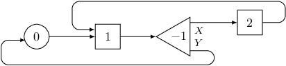
On the following picture there is a circuit with two triggers and one switch. Following connections of the circuit, we will visit triggers in order $1, 2, 1$.

Warmup

We start by solving subtask 1 in which every trigger appears in sequence $A$ at most once. Therefore we do not have to use any switches, we just connect triggers in the required order.

First of all, we can treat the origin as a trigger, and put its device number at the beginning (or at the end, it does not matter) of sequence $A$. Then for every trigger $i$ that appears in the sequence, we connect its exit $C[i]$ to the next trigger in the sequence. We don't use any switches, so we left vectors $X$ and $Y$ empty.

In subtask 2 we can have triggers that appears twice in sequence $A$. Suppose that trigger $i$ appears at positions $j_0$ and $j_1$ in the sequence. Then we can connect the exit of this trigger to a switch, the exit X of this switch to trigger $A[j_0+1]$ and the exit Y of this switch to trigger $A[j_1+1]$.

First of all, for each trigger $i$ we create list $after[i]$ containing numbers of triggers that appear after trigger $i$ in sequence $A$. Then for every trigger, if it appears exactly once in the sequence (thus list $after[i]$ has length $1$), then we just connect it to $after[i][0]$). Otherwise we create a new switch (by increasing number of used switches $S$) and connect its exits to $after[i][0]$ and $after[i][1]$.

More than two appearances

In subtask 3 each trigger can appear up to four times. Let's think what to do with a trigger than appears exactly four times. We can create the following gadget using three switches positioned in two layers:

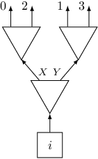
Such a gadget has four exits numbered from $0$ to $3$, exit $j$ will be connected to trigger $after[i][j]$. Note the order of exits on the picture.

What about a trigger that appears exactly three times? One could think that we can create a gadget using two switches, like the one on the left of the following picture:

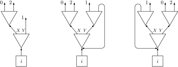
Unfortunately, such a gadget does not work, since it creates a sequence of triggers $0, 1, 2, 1$. A good idea is to use previous gadget with four exits, but to “kill” one of its exits, by connecting it to the bottom layer (see the middle picture). That would almost work, but there is a subtle catch here: if we kill the last exit, we would visit all triggers in the correct order, but we won't visit every switch an even number of times (and this was also a requirement in this problem). But killing any other exit is fine (for instance killing the first one, like in the right picture). In the code we need to add another if to handle sizes up to four:

The above idea can be generalized to solve the whole problem. If trigger $i$ appears $s$ times, we need to create a gadget $G_s$ that has exactly $s$ exits, connect trigger $i$ to this gadget, and connect the exit number $j$ of this gadget to $after[i][j]$. The function generate(after, S, X, Y) creates a desired gadget, updating values S, X and Y, and returns the number of device which is at the bottom of the gadget:

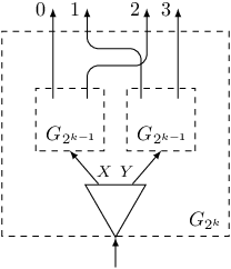
Suppose we need to create a gadget $G_s$ for $s=2^k$. We can construct it recursively from one switch and two gadgets $G_{2^{k-1}}$. The exits of gadget $G_{2^k}$ will be just exits of these two gadgets shuffled:

For value $s$ that is not a power of two, we find number $k$ such that $s \leq 2^k < 2s$. Then we create gadget $G_{2^k}$ and kill $2^k-s$ of its exits. The code is as follows:

Observe that we use array $revbits[j]$ to store the number $j$ after reversing the order of its bits, when expressed in binary form. It is useful, since the $j$-th exit from the left in the gadget $G_{2^k}$ is exit number $revbits[j]$. When choosing exits to kill, we take these whose numbers $revbits[j]$ are smaller than $2^k-s$. Thanks to that the remaining exits will have consecutive numbers, and we can connect exit of number $revbits[j]$ to trigger number $after[revbits[j] - (2^k - s)]$.

This solution uses at most $2s-1$ switches for a trigger that appears $s$ times in sequence $A$. Thus it uses at most $2N$ switches in total, which is enough for getting half score for subtasks 5 and 6.

The problem is that we use too many switches if $s$ is not a power of two. One idea how to handle it, is use a better way of killing unused exits. So far we killed exits with consecutive numbers, but it's better to kill exits that are located close to each other on the picture. Let's see an example with $s=5$ and $2^k=8$. If we kill the first three exits on the left, then one switch becomes unnecessary, since both of its exits will go to the bottom layer. Therefore, we can remove this switch:

This is easier said than done, since we need to know which switches to remove, and also we need to maintain correct order of connections on remaining exits. Perhaps recursive implementation would be more straightforward here, but nevertheless it can be implemented iteratively:

This way we use only $s + k-1$ switches. Therefore for subtask 5 in which we have only one trigger, we use less than $N + \log_2 N$ switches, as required for full points.

Unfortunately, this still does not give us full points for subtask 6, since we can get additional logarithmic addend for more than one trigger, and we won't fit in the switch limit. But it turns out that we do not need a separate gadget for every trigger. Indeed, we need only one gadget of size $N+1$. All triggers are connected to this gadget, and $N+1$ exits of the gadget are connected to triggers in the order they appear in sequence $A$:

This solution uses at most $N + \log_2 N$ switches and solves the whole problem.

As an author of this task, I can reveal that it was inspired by a certain mechanics in a puzzle computer game SpaceChem by Zachtronics. So if you have enjoyed solving it, you could enjoy playing the game.

Highway Tolls

In this problem we are given a connected undirected graph with $N$ vertices and $M$ edges. The vertices are numbered from $0$ to $N-1$. We are also given two constants $A$ and $B$ (satisfying $1\leq A < B$).

Two vertices $s$ and $t$ are chosen, but unknown to us, and we must guess them. In order to do that we can do the following procedure several times: we can arbitrarily assign weights $A$ and $B$ to the edges of the graph, turning it into a weighted graph. Then, we can ask what is the minimal possible weight for a path between $s$ and $t$ in this weighted graph. We do this by calling function ask, and we can only do a limited number of such calls.

The graph is a tree

When we are investigating paths in a graph, it is easier to deal with a tree, since in a tree there is a unique path between every two vertices.

One simple observation is that we can easily determine the length of the path $p$ between secret vertices $s$ and $t$ (that is the number of edges on the path between $s$ and $t$). If we assign equal weights of $A$ to all the edges of the graph, and function ask returns that the weight of path $p$ is equal to $W$, then the number of edges on the path is equal to $W/A$.

Another simple idea: we can determine if a certain edge $e$ belongs to path $p$. We just assign weight $B$ to this edge, and weight $A$ to all other edges. Now if edge $e$ does not belong to path $p$, the weight of this path is still $W$. Otherwise, the weight of path $p$ will be different (in fact it will be $W-A+B$).

If we apply such a test to every $N-1$ edges in the tree, we will determine all edges that belongs to path $p$, so in fact we will determine the whole path. The vertices $s$ and $t$ are the only vertices which are incident to exactly one edge from this path.

This code guesses vertices $s$ and $t$ after asking $N$ questions, and solves subtask 1.

Now we can move to subtask 3. The graph is no longer small, but it has even simpler structure: it is a line on which vertices are located in increasing numbers: $0, 1, \ldots, N-1$. Since the amount of questions we can ask is limited by $60$, the good intuition would be that we need to use some kind of binary search.

Indeed, since the edges on the line are ordered, we can use binary search to locate the first edge $e$ on path $p$. We do this as follows: we assume that this edge is located in range $[lb,ub]$. Then we split this range into $[lb,mid] \cup [mid+1,ub]$ and we assign to every edge from the left range weight $B$, and to remaining edges weight $A$. If weight of the path is greater than $W$, then we know, that at least one edge from path $p$ is located in the left range (so we can recurse to it), otherwise the first edge from $p$ is located in the right range:

When we find edge $e$, we know that the left endpoint of this edge will be vertex $s$. And since we have already determined the distance $W/A$ between vertices in one question, we know that $t = s+W/A$. The algorithm uses only $1 + \log_2 N$ questions.

In subtask 2 the tree is no longer a line, but we are given vertex $s$ for free. Thus we only need to find vertex $t$. Probably using binary search it is also a good idea. So let's try to find the edge on path $p$ that is furthest from vertex $s$. We can order all edges in such a way that edges that are closer to $s$ in a tree get smaller numbers than edges further from $s$. And then we can use similar binary search as on the line.

To get an ordering we can use either BFS (we can order the edges according to their distance from $s$) or DFS (we can order them according to the moment in time when we visit them). In the following code we use the latter approach:

First of all, we create the adjacency lists for the graph. Each list $adj[v]$ stores pairs $(e,u)$ for every edge $e = (v,u)$ of the graph. We also use additional array edge in which we store the numbers of edges as we traverse them with DFS, and also variable E to track the number of already traversed edges. Moreover, in vert[e] we store the endpoint of edge $e$ which is further from $s$. So if $el$ will be the last edge on path $p$, we return $t = vert[el]$:

The last part is function get_last_edge. It is very similar to get_first_edge, but know we are doing it backwards. Note that this function could return $-1$ if the path has zero length. This cannot happen now, but it will become useful later. Note also that this function does not need to know the length of path $p$.

Overall, we can solve subtask 2 using $1 + \log_2 N$ questions.

In subtask 4 we have a tree without any additional hints. But we already have experience in binary search, so why not use it once more? We know that if we impose some arbitrary order on the edges, we can use binary search to find the edge from path $p$ with the smallest number. In particular it means that we can find some edge $e=(u,v)$ on path $p$. If we remove this edge, the tree will separate into two subtrees of roots $u$ and $v$ respectively. We know that vertices $s$ and $t$ are in different trees, so we can treat them as separate problems.

In the first tree rooted in $v$ we need to find vertex $s$. Observe that path from $v$ to $s$ is part of path $p$. So we can use solution from subtask 2 to find the last edge on this path, if we assign weight $A$ to all edges outside the subtree. In a similar way we can find vertex $t$ in the second subtree:

When calling dfs function, we assign $u$ as the parent of vertex $v$, so we won't traverse edge $(v,u)$, and we only traverse subtree rooted at $v$. Note that this time function get_last_edge can return $-1$, which means that $v$ is one of the endpoint of path $p$.

The solution uses at most $1 + 3\log_2 N$ questions. But actually this is not the best upper bound we can get. Note, that two subtrees on which we are calling function get_last_edge are smaller than $N$ vertices, in fact they have $N_1$ and $N_2$ vertices respectively, where $N=N_1+N_2$. Thus we need $\log_2 N_1 + \log_2 N_2$ questions for them and that function achieves maximum for $N_1=N_2=N/2$, thus we need at most $2\log_2 \frac{N}{2} = 2(\log_2 N - 1)$ questions. Therefore for the whole algorithm we need $3\log_2 N - 1$.

Constants have different parity

Now let's move to subtask 5. This time the graph does not have to be a tree, but the constants are fixed to $A=1$ and $B=2$. In fact, the important thing about them is that they are of different parity.

Consider a following question: suppose that we have partitioned the set of all vertices in the graph into two subsets $V_1$ and $V_2$. Can we tell whether vertices $s$ and $t$ belong to the same set or different sets?

It turns out that we can. We assign odd weight $A$ to every edge that connects vertex from subset $V_1$ to a vertex from subset $V_2$. To the remaining edges (that connects vertices inside one subset), we assign even weight $B$. We can see that every path that starts in vertex from $V_1$ and ends in vertex from $V_2$ must contain an odd number of edges of weight $A$, since it must traverse between subsets odd number of times. Therefore the weight of this path is odd. Conversely, every path that starts and ends in the same subset, must contain an even number of edges of weight $A$, thus its weight is even.

The function that does that is simple. The argument grp is a vector of length $N$, where grp[i] is equal to 0 or 1 depending if vertex $i$ belongs to $V_1$ or $V_2$:

We could use this idea to test whether a certain vertex $v$ was chosen as $s$ or $t$. It is enough to consider $V_1=\{v\}$, and if $s$ and $t$ belong to different sets, we know that $v$ must be one of them. Unfortunately, to test all vertices this way, we would use $N$ questions, which is way too much to solve subtask 5.

But suppose that we have found two subsets $V_s$ and $V_t$ such that one of them contains vertex $s$, and the other one contains vertex $t$. Then we can use binary search to find vertex $t$: we can partition $V_t$ into two subsets $V_{t,1}$ and $V_{t,2}$ of roughly the same size, and ask question about subsets $V_s \cup V_{t,1}$ and subset $V_{t,2}$. If function returns same group, then we know that $t$ must be in subset $V_{t,1}$, otherwise $t$ must be in subset $V_{t,2}$. This way we reduced the size of subset containing $t$ by half. Thus after $\log_2 N$ steps we will reduce it to one vertex. The below code does this, assuming that vector grp_diff contains initial partition:

The same way we can do to find vertex $s$, and it also will cost $\log_2 N$ questions. So the last thing is: how to find an initial partition into $V_s$ and $V_t$? There is a nice trick to do this, that requires to consider only $\log_2 N$ candidate partitions. In the $i$-th candidate we partition the vertices according the $i$-th bit in their number: all vertices with this bit set to $0$ go into subset $V_s$, and all vertices with bit set to $1$ go into subset $V_t$. Note that since $s\neq t$, there is at least one bit on which they differ, so at least one candidate partition will satisfy our requirement.

So the code is as follows:

Overall we will ask at most $3\log_2 N$ questions, so since $\log_2 N \leq 17$, we will fit under limit of $52$ questions for subtask 5.

We can improve the above solution, so it only asks $2\log_2 N$ questions. In the first part we will consider $\log_2 N$ candidates, depending on the bits. Thanks to that we can compute $x = s \mathop{\mathrm{xor}} t$.

Now we know that if vertex $v$ was chosen, then the other chosen vertex must be $v \mathop{\mathrm{xor}} x$. So if we if use $\log_2 N$ question to determine vertex $s$, we immediately know that $t = s \mathop{\mathrm{xor}} x$. The code is as follows:

General problem

In graph that is not a tree there can be more that one shortest path between vertices $s$ and $t$. But even then we can use binary search to find an edge $e$ that lies on one of these shortest paths.

We can think about it as follows: at the beginning all edges have weight $A$. Then we proceed in turns, in each turn we change the weight of some edge from $A$ to $B$ and see whether the weight of a shortest path in weighted graph increased. If yes, that means that the latest edge changed must lie on a shortest path from $s$ to $t$. Of course, we can implement this idea efficiently, using binary search. That is exactly what function get_first_edge is doing.

That means that we have an edge $e$ on some shortest path from $s$ to $t$. Let's consider vertex $v$ incident with this edge; that means that $v$ lies on a shortest path from $s$ to $t$. Now we run a BFS to obtain a tree of shortest paths from vertex $v$ and order all edges in this tree according to their distance from vertex $v$. Based on this order we can use get_last_edge function to find the vertex $s$.

There is one subtle point here. Since shortest paths are not necessarily unique, and we need a tree for get_last_edge function, we need to assign weight $B$ to all edges which belong to some shortest path, but do not belong to BFS tree.

After running this algorithm, we rerun it constructing a BFS from vertex $s$. This way we will find vertex $t$. The code is as follows:

We use $1 + 3\log_2 N$ questions, so that why we get partial points on subtask 6. To get full points we need to remove at least $2$ questions, to get $3 \log_2 N - 1$, so we probably need a “partition” solution we used in subtask 4.

We know that can find an edge $e = (u,v)$ on a shortest path from $s$ to $t$. Without loss of generality, we can assume that vertices $s$, $u$, $v$ and $t$ appears in this order on this path. Then we can see that vertex $s$ is strictly closer to $u$ than $v$, otherwise edge $(u,v)$ could not lie on a shortest path from $s$ to $t$. Similarly, $t$ is closer to $v$ than to $u$.

That means that if we consider the set $S$ of all vertices that are closer to $u$ than $v$, and the set $T$ of all vertices that are closer to $v$ than $u$, then these sets are disjoint, set $S$ contains $u$ and $s$, and set $T$ contains $v$ and $t$. Moreover, we can construct BFS trees on the sets $S$ and $T$, rooted in $u$ and $v$ respectively, and the shortest path will go through edge $e$ and edges in BFS trees.

There is another subtle point here: since shortest paths are not unique, there could be some shortest paths from $s$ to $t$ that do not contain edge $e$. But that means that such a path will contain an edge that does not belong to $T$ nor $S$, so we can just assign weight $B$ for all such edges. The code is as follows:

The above code solves all subtasks using at most $3\log_2 N - 1$ questions.

Meetings

In this problem we are given a sequence of integers $H_0, H_1, \ldots, H_{N-1}$ of length $N$ and $Q$ queries. Each query is represented by a pair of integers $(L,R)$ and we must find a position $x$ in range $[L,R]$ that minimizes the sum

$cost_{L,R}(x) = \sum_{L\leq k \leq R} maxH(x,k),$

where $maxH(x,k)$ denotes the maximum value of $H_i$ between indices $x$ and $k$ (inclusive).

Trying every possible position

First, let us see how to solve just a single query $(L,R)$. The easiest way is to iterate over all possible positions $x$ and calculate $cost_{L,R}(x)$ independently for each of them. For $x \leq k$ we have that

$maxH(x,k) = \max_{x \le i \le k} H_i = \max(maxH(x,k-1), H_k)$.

Therefore we can calculate such values $maxH(x,k)$ by iterating $k$ from $x$ to $R$ and maintaining a running maximum. Similarly for $x \geq k$, so we can calculate values $maxH(x,k)$ for all $k$ in $O(R-L)$ time:

Since we have $Q$ queries, for each we test $O(N)$ candidates for value $x$ and for each candidate we calculate $cost_{L,R}(x)$ in $O(N)$, the total time complexity of this solution is $O(QN^2)$. This is enough to pass subtask 1.

To get a faster solution, we cannot calculate $cost_{L,R}(x)$ independently for each $x$. Instead, we split it into two parts for $k$ less than $x$ and $k$ greater than $x$:

$costL_{L,R}(x) = \sum_{L\le k < x} maxH(x,k),\qquad costR_{L,R}(x) = \sum_{x < k \le R} maxH(x,k).$

Of course, we have $cost_{L,R}(x) = costL_{L,R}(x) + H_x + costR_{L,R}(x)$. First, we calculate values $costL_{L,R}(x)$ by iterating $x$ from $L$ to $R$. Then, we similarly calculate values $costR_{L,R}(x)$ by iterating $x$ from $R$ to $L$.

Suppose that we have calculated $costL_{L,R}(x-1)$ and now we want to calculate $costL_{L,R}(x)$. Let $y$ be the first position to the left of $x$ such that $H_y > H_x$. Then the contribution of all heights in the range $[y+1,x]$ must be changed to $H_x$.

We use a stack to store information that are needed to make such changes. We call a position $y$ “visible” if all positions between $y$ and $x$ are smaller than $H_y$. On the stack we have pairs

$(h_1,c_1),\ (h_2,c_2),\ \ldots,\ (h_s,c_s)$

containing heights $h_1 > h_2 > \ldots > h_s$ on all visible positions. Value $c_i$ denotes number of positions between height $h_{i-1}$ and height $h_i$. The current contribution is a sum $\sum_i h_i \cdot c_i$.

Since every element is pushed on the stack at most once, the time complexity for each query is $O(N)$. So in total the algorithm works in $O(QN)$. This allows to pass subtask 2.

There is a simpler solution that passes subtask 2, but it requires some preprocessing. Observe that $costL_{L,R}(x)$ does not depend on $R$. Moreover, we can calculate these values for different $L$s by iterating from $x$ downwards and maintaining running maximum. Similarly we can do for $costR_{L,R}(x)$:

Such preprocessing runs in time $O(N^2)$. Now it is easy to use these values to answer queries in time $O(N)$ each:

So the total time complexity is $O(N^2 + QN)$.

Assuming small number of different heights

In subtask 3 we are told that the sequence of heights $H_i$ can have only two values: $1$ or $2$. In this case our problem is much simpler, since then

$cost_{L,R}(x) = 2(R-L+1)-longest_{L,R}(x),$

where $longest_{L,R}(x)$ is the length of the longest fragment that contains position $x$ and only positions with height $1$ (thus $longest_{L,R}(x)=0$ if $H_x=2$).

Therefore the answer to query $(L,R)$ is just $2(R-L+1)$ minus the longest fragment inside range $[L,R]$ that contains only positions with height $1$. Finding such a fragment is a classic problem that can be solved using a segment tree. The idea is that in each node of the tree we keep four values: best (longest fragment inside the range corresponding to this node), le (longest fragment that is a prefix of this range), ri (longest fragment that is a suffix of this range), len (the length of the range). You can read detailed explanation in my article about maximum-subarray problem, so here we only give C++ code for completeness:

The rest of the code is very simple:

Since the initialization of the tree runs in $O(N)$ time, and each query in $O(\log N)$ time, the overall time complexity of this solution is $O(N + Q\log N)$ that solves subtask 3.

In subtask 4 we have constraint that $H_i \leq 20$. Let us try to solve this subtask also with a segment tree. The idea is as follows: for a given fragment $[x_L,x_R]$ corresponding to some node in the segment tree we will calculate an array that stores the contribution from this fragment when we choose the position $x$ in this fragment. Value $cost[h_L,h_R]$ denotes the best contribution when

$h_L = \max_{x_L\leq i\leq x} H_i,\qquad h_R = \max_{x\leq i\leq x_R} H_i$.

To update these values we need also two additional arrays that store the contribution from the fragment when the chosen position $x$ is outside of the fragment. Value $le[h]$ denotes the contribution when fragment is to the left of position $x$ and the maximal height between fragment and the position is $h = \max_{x_R < i\leq x} H_i$. Similarly value $ri[h]$ denotes the contribution when fragment is to the right of $x$ and $h = \max_{x\leq i < x_L} H_i$.

Additionally, we store the maximal height in the fragment $maxh = \max_{x_L\leq x\leq x_R} H_i$. The structure and code for a fragment of length $1$ is simple:

The join function that combines values stored for the left half and the right half of a fragment into information about the whole fragment is more involved. To calculate costs we have to consider two cases: the chosen position $x$ is either in the left half or it is in the right half. In the former case, we iterate over all possibilities of values $cost[h_1,h_2]$ for the left fragment and combine it with the contribution from the right one, which is of course $ri[h_2]$. That gives us an obtainable cost for the whole fragment where $h_L = h_1$ and $h_R = \max(h_2, R.maxh)$. In the later case we have symmetric code.

Code to update arrays $le$ and $ri$ is even simpler. The whole function join could look as follows:

The rest of the code for the segment tree is the same as in the previous algorithm. To answer a query we just iterate over all possible costs for a given fragment:

Each structure info2_t stores $O(H^2)$ values (where $H = 20$), and this is the time of initialization this structure. Also, time complexity of join function is $O(H^2)$. Therefore the whole algorithm works in time $O(H^2(N + Q\log N))$.

We left as an exercise speeding-up this code to run in time $O(H(N + Q\log N))$. The crucial observation is that we only fill values $cost[h_L,h_R]$ if either $h_L$ or $h_R$ (or both) is equal to the maximal height in the fragment. Therefore we have only $O(H)$ interesting cells to fill in the array. This complexity is enough to solve subtask 4.

There is another solution for this subtask. In the previous one we split the sequence evenly, building a segment tree, thus in every node we needed to store information about various heights. In the next algorithm we will split this sequence based on the heights, so hopefully information we will need to store in the nodes of the tree will be simpler. The price we will have to pay for this will be increase in the height of the tree.

Each node of the tree contains information about some fragment $[x_L,x_R]$, but since we split them not necessarily in half, we store $x_L$ and $x_R$ in the node. We store also position $x_H$ of a point in which we split this fragment in two parts: left part $[x_L,x_H-1]$ and right part $[x_H+1,x_R]$ (we exclude position $x_H$ from these parts). We also store pointers to these two parts and the value $best$ that denotes the best possible cost if the position $x$ is chosen inside the fragment.

We always split the fragment in such a way that position $x_H$ contains the highest value in the fragment. If there is more than one position with the highest value, we split the fragment in the “middle” highest value, i.e. the number of highest values in the left and the right part differ at most by one.

Suppose we recursively solve the left and the right part, and we want to calculate best cost for the whole fragment. Again, we have two cases: either position $x$ is in the left part or in the right part. In the former case we add best cost from the left part to the contribution from the right part. But since the height in position $x_H$ is no less than any height in the right part, the contribution from the right part is just $H_{x_H}$ multiplied by the length of this part. We solve the latter case symmetrically:

The crucial point is to estimate the height of the tree. For every node we can assign a pair $(h,c)$ which means that in the fragment corresponding to this node the maximum height is $h$ and we have exactly $c$ positions with this maximum height. Every time we descend from a node to its child, we either go to $(h,c/2)$ reducing the number of maximal positions by half, or we go to $(h',c')$ where $h' < h$ and $c' \leq N$, reducing the maximal height. Therefore the length of each path is limited by $O(H \log N)$. Thus procedure that creates the tree takes $O(NH\log N)$.

To query the tree for a certain fragment, we descend recursively from the root. We will visit at most two paths of this tree, just like in code for query in a segment tree:

Finally the code to answer a query:

The overall complexity of this solution is therefore $O(H(N\log N + Q\log N))$.

Solving general problem

Now we are ready for the last subtask, whose solution will be the most involved among all. Let's consider a single query $[L,R]$. Let $v$ be a position inside this range with the greatest height $H_v$ (if there are more such positions, we choose the right-most one). The optimal chosen position $x$ for this query will be either to the right of $v$ or to the left of $v$ (it cannot be $v$ itself, since this would result in the worst possible cost of $H_v (R-L+1)$). We can consider the former case only (that $x$ is to the right of $v$) for all the queries, and then run the same algorithm once again on a reversed array $H$.

If the chosen position $x$ is to the right of $v$, then the best cost is equal to $H_v(v - L + 1)$ plus the optimal cost for range $[v+1,R]$. To quickly find position $v$ in range $[L,R]$ we can use any solution to Range Maximum Query problem discussed before, for instance a segment tree. In the nodes of this segment tree we will store not just values $H_i$, but pairs $(H_i,i)$. Thanks to that we will be able to easily break ties with equal heights, and also the resulting maximum pair will contain both height $H_v$ and its position $v$. The solution could look like this (parts of the code in italics will be explained later):

It may look like we haven't gained anything, since we still need to calculate the optimal cost for range $[v+1,R]$. But this is not a general case, since we know that $H_v$ must be greater than any value in this range.

As in the previous algorithm, we try a solution with partitioning based on heights. Let $H_v$ be the highest element in the sequence. We will build a tree with $v$ in the root and pointers to left and right children that contains trees recursively created for ranges $[0,v-1]$ and $[v+1,N-1]$. This structure is called Cartesian tree and we can build it in $O(N)$ time using different algorithms. We can for instance use divide and conquer approach:

Each node in the tree is described by a structure node2_t that has, among others, fields: x (position in the sequence), L and R (pointers to the left and the right child). The other fields will be explained later.

Let's consider a position $v$ with height $H_v$. Let $v_L$ be the left-most position such that all heights in range $[v_L,v-1]$ are smaller than $H_v$. Similarly denote $v_R$ as the right-most position such that all heights in range $[v+1,v_R]$ are smaller than $H_v$. The nodes in the left subtree of $v$ in the Cartesian tree are exactly nodes from range $[v_L,v-1]$, similarly the nodes in range $[v+1,v_R]$ are from the right subtree of $v$. Having a Cartesian tree we can easily calculate values $v_L$ and $v_R$ for all nodes in $O(N)$. We store them in fields xl and xr of the structure:

Moreover, we fill array nodes which store for every position in the sequence corresponding node in the Cartesian tree.

Finally we are able to explain, which cost values we will be calculating. For every node $v$ we will create an array $S_v$ of length $v_R-v_L+1$ such that value $S_v[i]$ denotes optimal cost for the range $[v_L,v_L+i]$ (where $0 \leq i \leq v_R-v_L$). We will calculate array $S_v$ based on arrays $S_{L_v}$ and $S_{R_v}$, where $L_v$ and $R_v$ denotes left and right child of $v$, respectively. We will do this in a destructive manner, i.e. calculation of array $S_v$ will destruct arrays $S_{L_v}$ and $S_{R_v}$. Therefore we must use all information in array $S_v$ as soon as we construct it.

Recall that we need to calculate optimal cost for range $[v+1,R]$ where $H_v$ is greater than any height in this range. Thus if we consider array $S_u$, where $u=R_v$ is the right child of node $v$, it will contain this cost in the element $R-v-1$. Indeed, we have $u_L = v+1$ and $R \leq u_R$. Therefore we will note that as soon as this array is available, we would like to use it. So for every node in the tree we will have a vector of queries that contains pairs of index in the array we are interested in and pointer to where to put this index. We fill this array in this line:

Now we need to construct array $S_v$ based on $S_{L_v}$ and $S_{R_v}$. We can partition array $S_v$ into three parts of lengths $v-v_L$, $1$, and $v_R-v$ respectively. Clearly, values in the left part will be exactly the same as values in array $S_{L_v}$. The middle value will be the cost of $[v_L,v]$, which since $H_v$ is the highest, is equal to cost of $[v_L,v-1]$ (last element in $S_{L_v}$) plus $H_v$. Time for right values.

Let's consider the cost for range $[v_L,v+1+i]$ for $0 \leq i < v_R-v$. We have

$cost[v_L,v+1+i] = \min( f(i), g(i) ),$

where $f(i)$ denotes the cost if chosen position $x$ is to the left of $v$, and $g(i)$ denotes the cost if $x$ is to the right of $v$. We can describe them as follows:

$f(i) = cost[v_L,v-1] + (2+i)H_v$,

$g(i) = (v-v_L+1)H_v + cost[v+1,v+1+i],$

thus $f(i)$ is a linear function with slope $H_v$ and intercept $cost[v_L,v-1] + 2H_v$, and values of $g(i)$ are values in array $S_{R_v}$ increased by constant $(v-v_L+1) H_v$.

Consider now the difference $\Delta(i) = f(i) - g(i)$ between these functions. It turns out that this function is monotonic:

$\Delta(i+1)-\Delta(i) = f(i+1)-f(i)-g(i+1)+g(i) =$

$\qquad\qquad\qquad\quad = H_v - cost[v+1,v+1+(i+1)] + cost[v+1,v+1+i] \geq 0.$

The last inequality follows from the fact that extending range $[v+1,v+1+i]$ by one element cannot increase cost more than $H_v$ (since this is the largest height).

Since the difference $f(i)-g(i)$ increases, that means that the minimum $\min(f(i),g(i))$ is equal to $f(i)$ for some time, and then it is equal to $g(i)$, i.e. there is some position $j$ that

$cost[v_L,v+1+i] = \left\{\begin{array}{ll} f(i) & i \leq j, \\ g(i) & i > j. \end{array}\right.$

Thus if we find index $j$, then we can fill the right part of array $S_v$ as follows: up to $j$ we fill it according to linear function $f(i)$, and after this we fill it with values of $g(i)$ increased by some constant.

Of course, we cannot represent arrays $S_v$ directly, since that would result in $O(n^2)$ time complexity. So we use some compressed representation for them. We see that some part of $S_v$ can be represented by a linear function. This gives us an idea to represent whole $S_v$ as a piecewise-linear function, i.e. as a set of ranges (which we call fragments), and in each fragment function $S_v$ is linear.

We store all fragments in a map frags indexed by the first positions of each fragment. Apart from that each fragment stores its length and two parameters of the linear function. Member function eval simply evaluates linear function in a certain offset from the first position:

Storing all fragments in one map has two advantages. First, when creating left part of array $S_v$ by copying from $S_{L_v}$ we do not have to do anything, since all fragments representing $S_{L_v}$ are already in the map. Second, we can easily evaluate the $i$-th index in created $S_v$, by performing one binary search on position $v_L+i$ in this map in $O(\log N)$ and evaluating one linear function. That means that we can answer all queries in total time of $O(Q\log N)$.

To calculate the middle value in $S_v$ is enough to evaluate the last position in $S_{L_v}$ and add $H_v$ to it.

That leaves us with calculating the right part of $S_v$. First, we create new fragment $F$ for linear function $f(i)$. Then, we find index $j$ by comparing $f(i)$ with fragments representing $S_{R_v}$. Let's denote by $G$ the first such fragment. As long as the value of the last position in $G$ is greater than the value of the same position in $F$, we know that on the whole range of $G$ function $F$ is smaller, so we remove $G$ completely. Finally, we either run out of fragments in $S_{R_v}$, or we find a fragment $G$ that intersects with $F$. In the latter case, we find index $j$ of the intersection (we can do it by using a formula or we can just take $O(\log N)$ time for a binary search), and we update length of $F$ (so it ends in $j$), and parameters of $G$ (so it starts in $j+1$).

Since every fragment is removed from the map at most once, all removals costs us $O(N\log N)$.

The last bit we need to do is to add certain constant to all the remaining fragments in $S_{R_v}$, before they become fragments of $S_v$. We do this by using lazy propagation strategy. Each node $v$ has two additional fields: frag_len denoting number of fragments that covers array $S_v$, and frag_off denoting the value that must be added to linear functions in all these fragments. So we can add any constant to all fragments in $S_{R_v}$ by adding it to frag_off in $R_v$.

So we have two bits left: now during each evaluation of a linear function, we must remember to what array this function belongs, and add appropriate value frag_off. And second: now array $S_v$ contains some fragments from $S_{L_v}$ and some fragments from $S_{R_v}$, and they probably have different values of frag_off, let's call them $off_L$ and $off_R$. In order to update them, so we can have common value $off$ for array $S_v$, we use a “merging smaller to bigger” trick. If array $S_{L_v}$ has less fragments than array $S_{R_v}$, we add value $off_L - off_R$ to linear functions in all fragments in $S_{L_v}$ and we set $off = off_R$. Otherwise, we update fragments in $S_{R_v}$. Since after update of a function its array increases at least twice, we will update this function at most $O(\log N)$ times, so the total time spending on updates will be $O(N\log N)$.

The full code of the calculate function is as follows:

Overall, the total time complexity is $O(N\log N + Q\log N)$ and that solution solves all subtasks.